Linear Regression (Python Implementation)

 

Linear regression is perhaps one of the most well known and well-understood algorithms in statistics and machine learning.

In this post, you will discover the linear regression algorithm, how it works, and how you can best use it in on your machine learning projects.

Contents…

•Linear Regression

•Simple Linear Regression

•Multiple Linear Regression

•Assumptions

•Applications

Linear Regression

A statistical approach for modeling relationship between a dependent variable with a given set of independent variables.

We refer dependent variables as response and independent variables as features

Simple Linear Regression

Simple linear regression is an approach for predicting a response using a single feature.

It is assumed that the two variables are linearly related. Hence, we try to find a linear function that predicts the response value(y) as accurately as possible as a function of the feature or independent variable(x).

Let us consider a dataset where we have a value of response y for every feature x:

A dataset

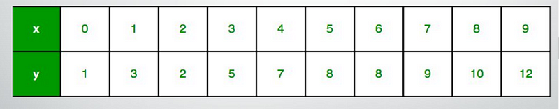
For generality, we define:

x as feature vector, i.e x = [x_1, x_2, …., x_n],

y as response vector, i.e y = [y_1, y_2, …., y_n]

for n observations (in above example, n=10).

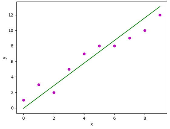
A scatter plot of a given dataset looks like:-

a plot of a given dataset

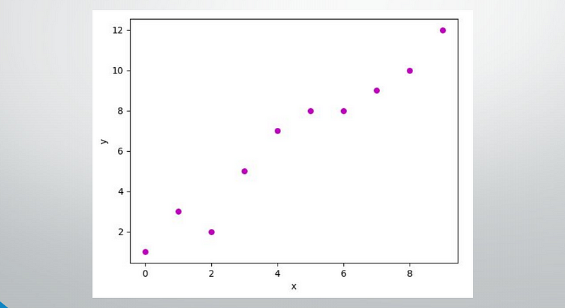
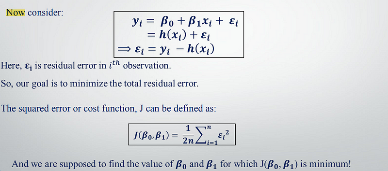
Now, the task is to find a line that fits best in the above scatter plot so that we can predict the response for any new feature values. (i.e. a value of x not present in the dataset) This line is called the regression line.

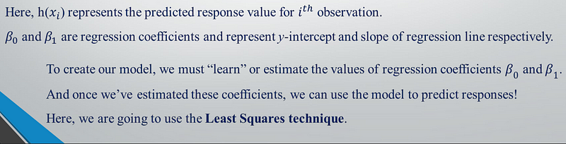
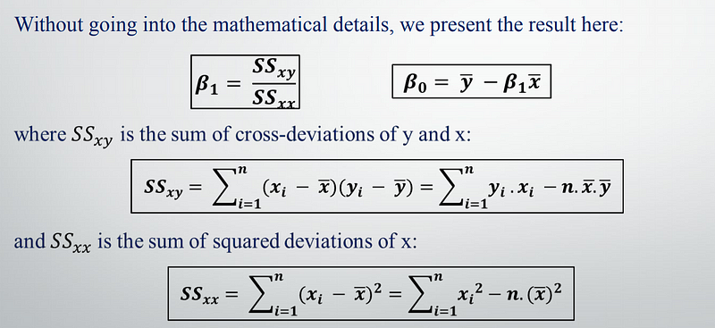
The equation of the regression line is represented as:

equation of the regression line

Given is the python implementation of the technique on our small dataset:

import numpy as np
import matplotlib.pyplot as plt
def estimate_coef(x, y):
# number of observations/points
   n = np.size(x)
# mean of x and y vector
   m_x, m_y = np.mean(x), np.mean(y)
# calculating cross-deviation and deviation about x
   SS_xy = np.sum(y*x - n*m_y*m_x)
   SS_xx = np.sum(x*x - n*m_x*m_x)
# calculating regression coefficients
   b_1 = SS_xy / SS_xx
   b_0 = m_y - b_1*m_x
   return(b_0, b_1)
def plot_regression_line(x, y, b):
# plotting the actual points as scatter plot
    plt.scatter(x, y, color = "m",
    marker = "o", s = 30)
# predicted response vector
    y_pred = b[0] + b[1]*x
# plotting the regression line
   plt.plot(x, y_pred, color = "g")
# putting labels
   plt.xlabel('x')
   plt.ylabel('y')
# function to show plot
   plt.show()
def main():
# observations
   x = np.array([0, 1, 2, 3, 4, 5, 6, 7, 8, 9])
   y = np.array([1, 3, 2, 5, 7, 8, 8, 9, 10, 12])
# estimating coefficients
   b = estimate_coef(x, y)
   print("Estimated coefficients:\nb_0 = {} \\nb_1 ={}"
   .format(b[0], b[1]))
# plotting regression line
   plot_regression_line(x, y, b)
if __name__ == "__main__":
  main()

The output of a given piece of code is:
 Estimated coefficients:
 β_0= -0.0586206896552
 β_1 = 1.45747126437

And the graph obtained looks like this:

In the next article, we will discuss Multiple Linear Regression.